
Nonlinear plate dynamics analysis based on FEM shell element with Absolute Nodal Coordinate Formulation (ANCF) 1. (This code is validated with MATLAB R2007b or later versions)

Language
Communication
Show Directories
├─Plate_FEM_explicit_3_SURFplot
│  ├─cores
│  │  ├─functions
│  │  ├─solver
│  │  └─ToolBoxes
│  └─save
│      └─fig
└─Plate_FEM_implicit_0
    ├─cores
    │  ├─functions
    │  ├─solver
    │  └─ToolBoxes
    └─save
        └─fig
-
Plate_FEM_implicit_0 : Implicit solver (Faster and more robust under the thin thickness condition)
-
Plate_FEM_explicit_3_SURFplot : Explicit solver (Light computing cost)
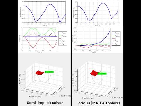
Comparisons between Semi-implicit solver vs ODE113 (MATLAB explicit solver)
This code with the implicit solver (Plate_FEM_implicit_0) was employed as a structure solver for the following publication(s):
Show Publications
- Influence of the aspect ratio of the sheet for an electric generator utilizing the rotation of a flapping sheet, Mechanical Engineering Journal, Vol. 8, No. 1 (2021).
https://doi.org/10.1299/mej.20-00459
@article{Akio YAMANO202120-00459,
    title={Influence of the aspect ratio of the sheet for an electric generator utilizing the rotation of a flapping sheet},
    author={Akio YAMANO and Hiroshi IJIMA and Atsuhiko SHINTANI and Chihiro NAKAGAWA and Tomohiro ITO},
    journal={Mechanical Engineering Journal},
    volume={8},
    number={1},
    pages={20-00459-20-00459},
    year={2021},
    doi={10.1299/mej.20-00459}
}
- Flow-induced vibration and energy-harvesting performance analysis for parallelized two flutter-mills considering span-wise plate deformation with geometrical nonlinearity and three-dimensional flow, International Journal of Structural Stability and Dynamics, Vol. 22, No. 14, (2022).
https://doi.org/10.1142/S0219455422501632
@article{doi:10.1142/S0219455422501632,
    author = {Yamano, Akio and Chiba, Masakatsu},
    title = {Flow-Induced Vibration and Energy-Harvesting Performance Analysis for Parallelized Two Flutter-Mills Considering Span-Wise Plate Deformation with Geometrical Nonlinearity and Three-Dimensional Flow},
    journal = {International Journal of Structural Stability and Dynamics},
    volume = {22},
    number = {14},
    pages = {2250163},
    year = {2022},
    doi = {10.1142/S0219455422501632}
}
- Influence of boundary conditions on a flutter-mill, Journal of Sound and Vibration, Vol. 478, No. 21 (2020).
https://doi.org/10.1016/j.jsv.2020.115359
@article{YAMANO2020115359,
    title = {Influence of boundary conditions on a flutter-mill},
    journal = {Journal of Sound and Vibration},
    volume = {478},
    pages = {115359},
    year = {2020},
    doi = {https://doi.org/10.1016/j.jsv.2020.115359},
    author = {A. Yamano and A. Shintani and T. Ito and C. Nakagawa and H. Ijima}
}
Show instructions
[Step 1] Install the ToolBoxes
The following ToolBoxes in “./XXXX/cores/ToolBoxes/” are required,
For numerical analysis:
- “Meshing a plate using four noded elements” by KSSV:
https://jp.mathworks.com/matlabcentral/fileexchange/33731-meshing-a-plate-using-four-noded-elements
- “Sparse sub access” by Bruno Luong:
https://jp.mathworks.com/matlabcentral/fileexchange/23488-sparse-sub-access
- “Vectorized Multi-Dimensional Matrix Multiplication” by Darin Koblick:
For plotting results:
- “mmwrite” by Micah Richert:
https://jp.mathworks.com/matlabcentral/fileexchange/15881-mmwrite
- “mpgwrite” by David Foti:
https://jp.mathworks.com/matlabcentral/fileexchange/309-mpgwrite?s_tid=srchtitle
- “mmread” by Micah Richert:
https://jp.mathworks.com/matlabcentral/fileexchange/8028-mmread
[Step 1.2] Add path to installed ToolBoxes
Modify "add_pathes.m" to add path to abovementined installed ToolBoxes as follows,
addpath ./cores/ToolBoxes/XX;
where XX is the name of folder of the installed ToolBox.
[Step 2] Start GUI form
Open the “GUI.fig” from MATLAB.

[Step 2.1] Pre-setting
Push the "Parameters" button and edit parameters.
[Step 3] Start analysis
Push the “exe” button and wait until the finish of the analysis.
[Step 4] Plot results
Push the “plot” button.
[Step 5] View plotted results
Results (figures and movie) plotted by [Step 4] are in "./save" directory.
Show instructions
Analytical condisions are in "./save/param_setting.m"
End_Time = 1.0;             %% Analytical time [s]
d_t = 1e-4;                 %% step time [s]
core_num = 6;               %% The number of CPUs for computing [-]
movie_format = 'mpeg';      %% movie format [-]
% movie_format = 'avi';
speed_check = 0;            %%

%% Plate
rho_m = 1000;           	%% density [kg/m^3]
Eelastic = 1e+3;        	%% Young's modulus [Pa]
nu = 0.3;                   %% Poiison ratio [-]

Length = 100e-3;          	%% Length [m]
Width = 100e-3;             %% Width [m]
thick = 10e-3;           	%% Thickness [m]
Nx = 8;                   	%% The number of x-directional elements [-]
Ny = 8;                   	%% The number of y-directional elements [-]
N_gauss = 5;                %% Gauss-Legendre [-]

g = 9.81;                   %% gravity acc. [m/s^2]
F_in = -rho_m*g*[ 0 0 1].';	%% gravity [N/m^3]
and boundary conditions for nodes on the plate;
%% Boundary conditions
node_r_0 = [ 1];          	%% Node number for fixed node [-]
node_dxr_0 = [ ];        	%% Node number for fixed x-directional gradient [-]
node_dyr_0 = [ ];       	%% Node number for fixed y-directional gradient [-]
Then, boundary conditions for a plate are written as,
- Pinned at the corner of the plate
%% Boundary conditions
node_r_0 = [ 1];          	%% Node number for fixed node [-]
node_dxr_0 = [ ];        	%% Node number for fixed x-directional gradient [-]
node_dyr_0 = [ ]; %% Node number for fixed y-directional gradient [-]- Clamped at the leading-edge
%% Boundary conditions
node_r_0 = [ 1:Ny+1 ];       %% Node number giving the displacement constraint [-]
node_dxr_0 = [ 1:Ny+1 ];     %% Node number giving x-directional gradient constraint [-]
node_dyr_0 = [ 1:Ny+1 ]; %% Node number giving y-directional gradient constraint [-]- Pinned at the leading-edge
%% Boundary conditions
node_r_0 = [ 1:Ny+1 ];     %% Node number giving the displacement constraint [-]
node_dxr_0 = [ ];          %% Node number giving x-directional gradient constraint [-]
node_dyr_0 = [ 1:Ny+1 ];   %% Node number giving y-directional gradient constraint [
where index in vector shows the node index around a plate element to apply boundary conditions.
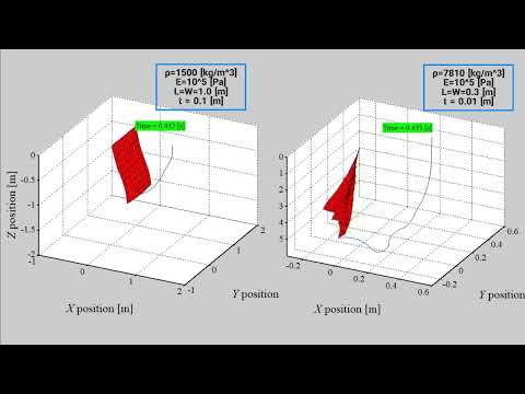
- Young's modulus:
$1.0 \times 10^5 \ \rm{Pa}$ - density:
$7810 \ \rm{kg/m^3}$ - Poisson ratio:
$0.3$ - Length, width:
$0.3 \ \rm{m}$ - Thickness:
$0.01 \ \rm{m}$

Deformed shape of the pendulum by this code (

Deformed shape of the pendulum by this code (

Deformed shape of the pendulum by the preceding report (Model I,

Time series of energy of the falling plate.

MIT License
Issue reports and pull requests are highly welcomed.