

trust-free is a Python package for fitting interpretable regression models using Transparent, Robust, and Ultra-Sparse Trees (TRUST™) — a new generation of Linear Model Trees (LMTs) with Random-Forest accuracy and intuitive explanations. It is based on my peer-reviewed paper [1], presented at the 22nd Pacific Rim International Conference on Artificial Intelligence (PRICAI 2025) and to appear in Springer Nature (Lecture Notes in Artificial Intelligence).
It includes a state-of-the-art explainability suite, providing comprehensive, automatically-generated explanation reports. To see it in action, here's a 30-second demo showcasing the explain() and compare() methods applied to the famous Medical Insurance Charges dataset from Kaggle:
| Model | Test R² ↑ | Interpretable? |
|---|---|---|
| TRUST™ | 0.67 | ✅ Yes |
| Random Forest (RF) | 0.62 | ❌ No |
| Lasso | 0.57 | ✅ Yes |
| CART | 0.49 | ✅ Yes |
| Node Harvest (NH) | 0.47 | ✅ Yes |
| M5' (Linear Model Tree) | 0.36 |
In the table above, TRUST™ is the only fully interpretable model statistically above 0.6 test R² across varied benchmark datasets — and 6× sparser than M5' (17 vs 109 coefficients on average).
Source: PRICAI 2025 (Springer LNAI)
Try it now on macOS or Linux: pip install trust-free. In Google Colab: %pip install trust-free.
See full benchmarks in the PRICAI 2025 paper
The package currently supports standard regression and experimental time-series regression tasks. Future releases will also tackle other tasks such as classification.
TRUST™ [1] is a next-generation algorithm based on (sparse) Linear Model Trees (LMTs), which I developed as part of my Ph.D. in Statistics at the University of Wisconsin-Madison. trust-free is the official Python implementation of the algorithm.
LMTs combine the strengths of two popular interpretable machine learning models: Decision Trees (non-parametric) and Linear Models (parametric). Like a standard Decision Tree, they partition data based on simple decision rules. However, the key difference lies in how they evaluate these splits and model the data. Instead of using a simple constant (like the average) to evaluate the goodness of a split, LMTs fit a Linear Model to the data within each node.
This approach means that the final predictions in the leaves are made by a Linear Model rather than a simple constant approximation. This gives Linear Model Trees both the predictive and explicative power of a linear model, while also retaining the ability of a tree-based algorithm to handle complex, non-linear relationships in the data. This way, LMTs can approximate well any Lp function in Lp norm, i.e. can learn almost any function. Importantly, the resulting fitted model is usually compact, making it easier to interpret.
Compared to existing LMT algorithms such as M5 [2], TRUST™ offers unmatched interpretability while approaching the accuracy of black-box models like Random Forests [3] — a combination that is rare in machine learning.
[1] Dorador, A. (2025). TRUST: Transparent, Robust and Ultra-Sparse Trees. arXiv:2506.15791.
[2] Quinlan, J.R. (1992). Learning with Continuous Classes. Australian Joint Conference on AI, 343–348.
[3] Breiman, L. (2001). Random Forests. Machine Learning, 45(1), 5–32.
-
Featured:
- Data Elixir (Issue 546) (over 60,000 subscribers)
- Data Science Weekly (Issue 616) (over 68,500 subscribers)
- University of Wisconsin - Madison Department of Statistics website (May 2025)
-
Upcoming Talks & Workshops:
- BarcelonaTech, Statistics Department (Dec 2025)
-
Past Talks & Workshops:
- PRICAI 2025 (Nov 2025)
- University of Seville, Minerva AI Lab (Oct 2025)
- Hybrid power: Trees to capture non-linearity & interactions + sparse linear (Relaxed Lasso) models in leaves
- Superior accuracy: RF-level accuracy, proven on 60 benchmark datasets
- Full transparency: Every prediction is auditable via tree path + leaf equation
- Inclusive: Explanation reports written in natural language accessible to all audiences
- Compliant by design: 100% Compliant with the EU AI Act and the OECD AI Principles — ideal for high-stakes domains like finance and healthcare
- ℹ️ Free-tier dataset limits: ≤ 5,000 rows and ≤ 20 columns (intended for proof-of-concept, R&D and teaching)
- ✅ All core features are fully functional within these bounds
- ✅ Unlimited scale and additional features in the forthcoming trust-pro edition
Want early access to trust-pro?
- Join the waitlist (completely anonymous & GDPR-compliant)
- Star ⭐ this repo to stay updated!
- Solves regression tasks (including a currently experimental 'time series mode')
- Interpretable models with accuracy comparable to Random Forests
- Visual tree structure and comprehensive, automatically-generated explanations on demand
- Automatically-generated head-to-head comparisons of profiles of interest
- Multiple variable importance methods (Ghost, Permutation, ALE plots, SHAP values)
- Automatic missing value handling that learns from missingness itself
- Automatic detection of potential overfitting.
- Ability to efficiently use continuous and categorical predictor variables
- Prediction confidence intervals [coming in next release]
- Novel method to warn about risky predictions on the fly [coming in next release]
- Novel in-leaf regression model delivering even further sparsity [coming in next release]
- Lightning fast training [coming in next release]
- Added:
- Expanded compatibility (new platforms will be sequentially added)
- Axis values in radar chart (compare method).
- Greedy feature order optimization (instead of exhaustive) in radar charts with more than 9 features.
- Pie and radar charts and saved to device in explain and compare method retain feature names when run in Jupyter too.
- Visual cues to convey training performance more easily.
- Automatic detection of potential overfitting.
- Changed:
- Changed prediction logic from recursive to iterative (more efficient).
- Reversed color scheme for bar chart in detailed mode for the compare method.
- Sorted dumbell plot from largest to smallest feature difference in compare method.
- Fixed bug in explain method for rare cases where no feature was statistically relevant.
- More accurate expected time to training completion after cross-validation.
- Swapped cosine similarity for angular similarity in compare() for more intuitive scaling.
- Other minor enhancements in explain() and compare() methods.
Check CHANGELOG.md to see all past release notes.
You can install this package using pip:
pip install trust-free📦 Note: The package name on PyPI is
trust-free, but the module you import in Python istrust:from trust import TRUST.
| Platform / Environment | OS & Arch | Python | Status |
|---|---|---|---|
| macOS ARM64 (M1–M4) | macOS 11+ ARM64 | 3.11–3.12 | ✅ Working |
| macOS Intel (x86_64) | macOS 11+ Intel | 3.11–3.12 | ✅ Working |
| Linux Intel/AMD | manylinux x86_64 | 3.11–3.12 | ✅ Working |
| Google Colab | Linux x86_64 | 3.12 | ✅ Working |
| Kaggle Notebooks | Linux x86_64 | 3.11 | ✅ Working* |
| Linux ARM64 | manylinux ARM64 | 3.11–3.12 | ✅ Working |
| Windows Intel/AMD | Windows 11 x86_64 | 3.11–3.12 | ✅ Working |
*If Kaggle shows a dependency-compatibility issue message upon installation via %pip install trust-free you may safely ignore it and hit "Restart and run up to selected cell" (assuming your selected cell is the one installing trust-free).
For a fully reproducible development environment with all dependencies, see SETUP.md.
Here are two basic examples of how to use the TRUST™ algorithm:
from trust import TRUST # note the import name is trust, not trust-free
from sklearn.datasets import make_regression
from sklearn.model_selection import train_test_split
from sklearn.metrics import r2_score, mean_squared_errorX, y, coefs = make_regression(n_samples=5000, n_features=20, n_informative=10, coef=True, noise=0.1, random_state=123)
print(coefs)
# x2 = 80.9
# x3 = 91.4
# x7 = 64.1
# x8 = 44.6
# x10 = 96.2
# x12 = 90.5
# x14 = 45.3
# x17 = 39.8
# x18 = 90.6
# x19 = 33.2
X_train, X_test, y_train, y_test = train_test_split(X, y, test_size=0.2, random_state=123)
# Instantiate and fit your model
model = TRUST()
model.fit(X_train, y_train)
# Predict and print results
y_pred = model.predict(X_test)
print("Predictions:", y_pred[:5])
print("True y values:", y_test[:5])
print("test R\u00B2:", r2_score(y_test, y_pred))# Obtain (conditional) variable importance by Ghost method (based on Delicado and Pena, 2023)
model.varImp(X_test, y_test, corAnalysis=True, filename="Synthetic")
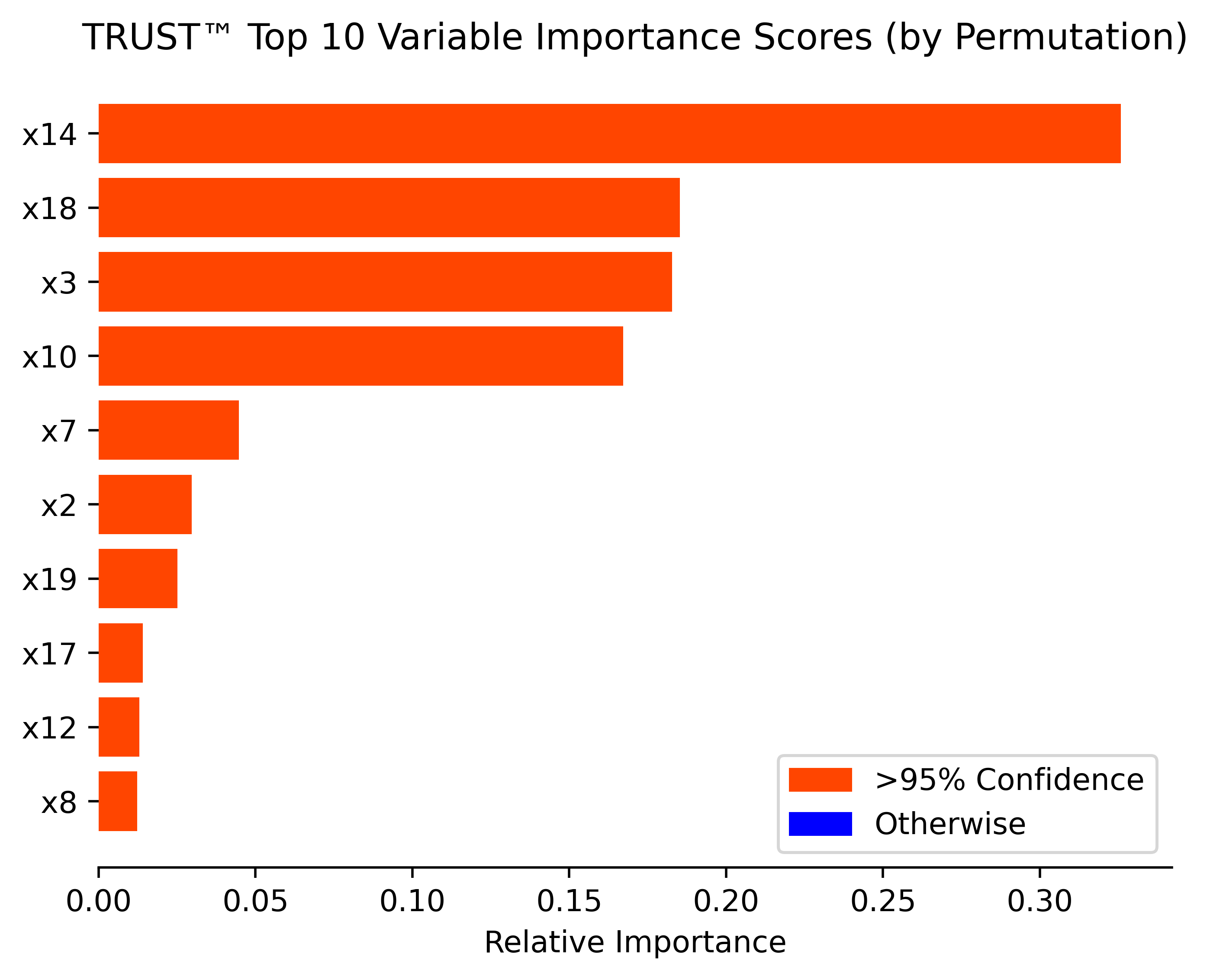
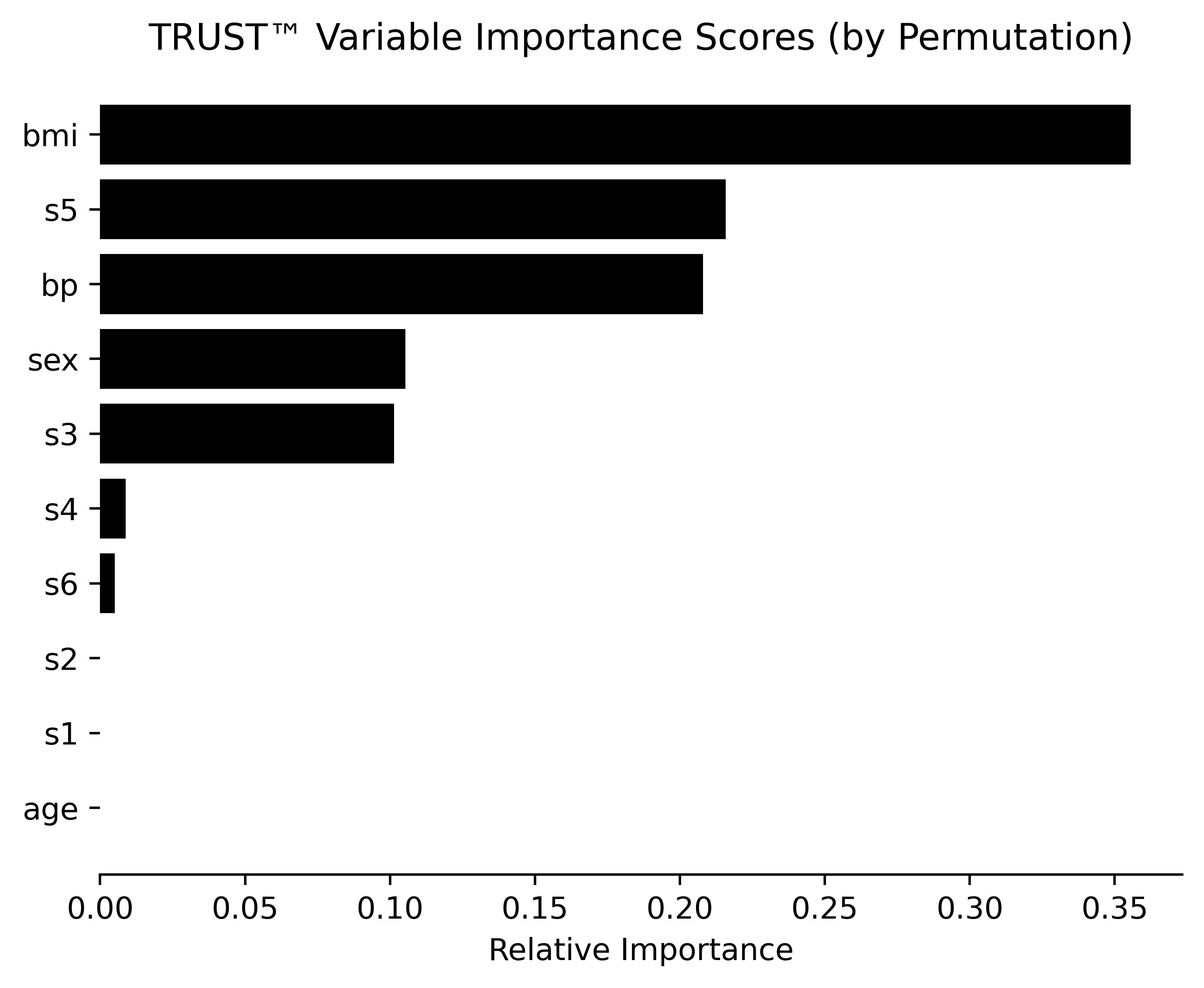
# Unconditional variable importance by permutation (with added debiasing and uncertainty quantification steps)
model.varImpPerm(X_test, y_test, R=20, B=20, U=10, filename="Synthetic")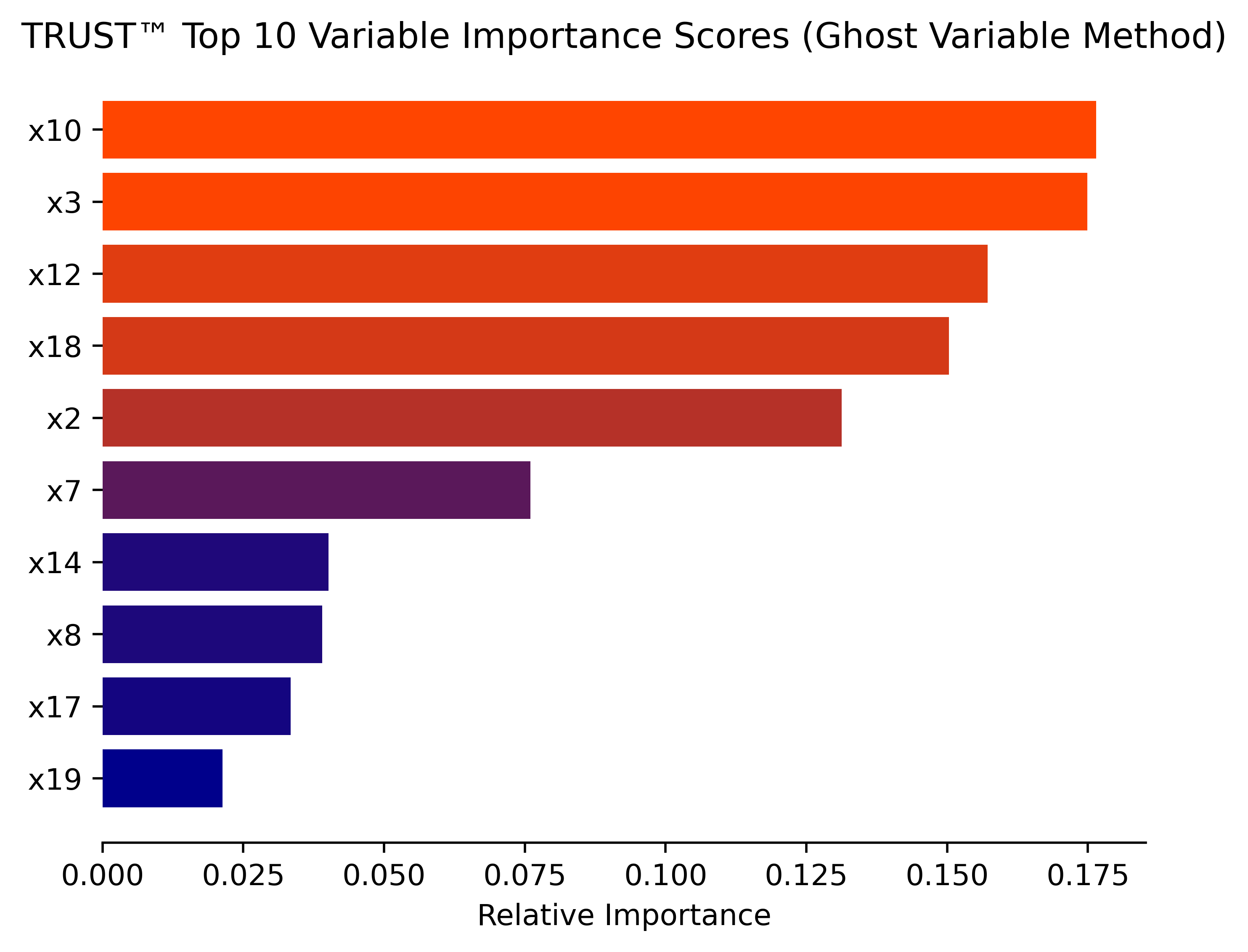
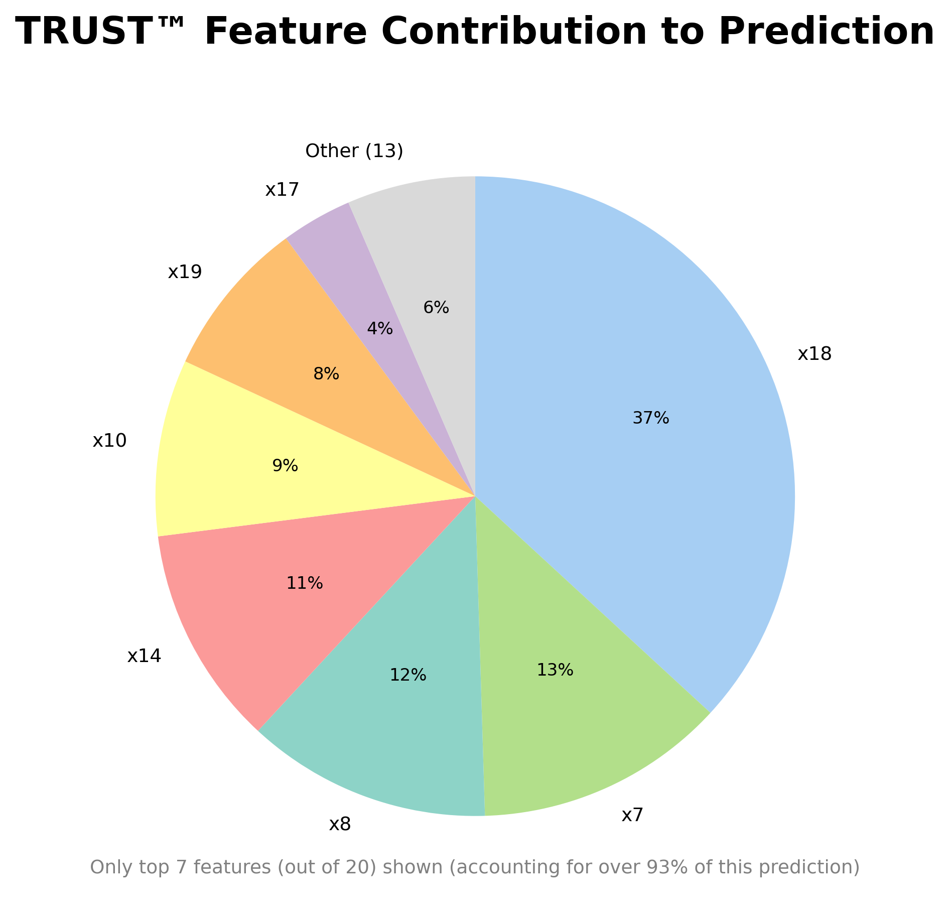
# Obtain prediction explanation for first observation
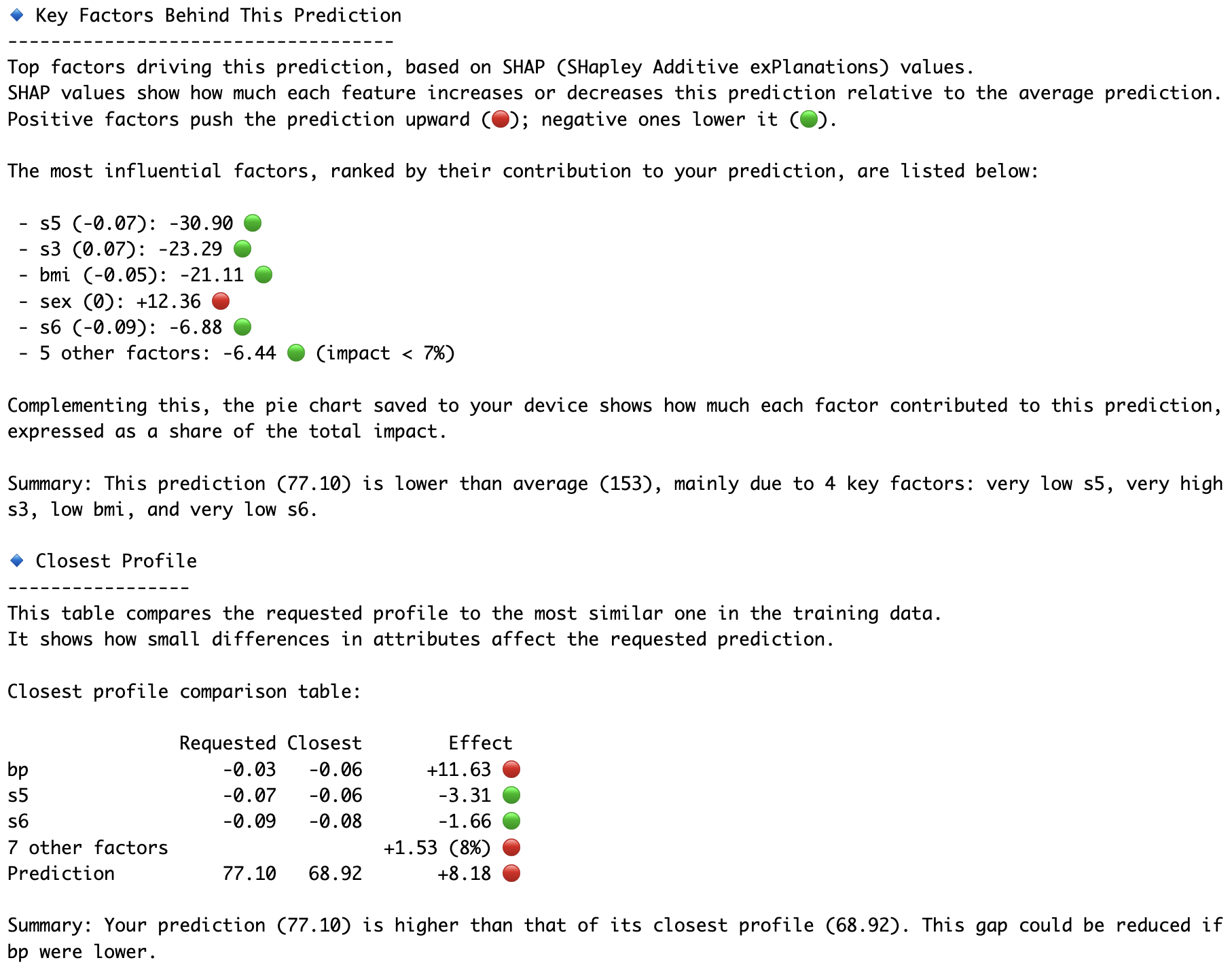
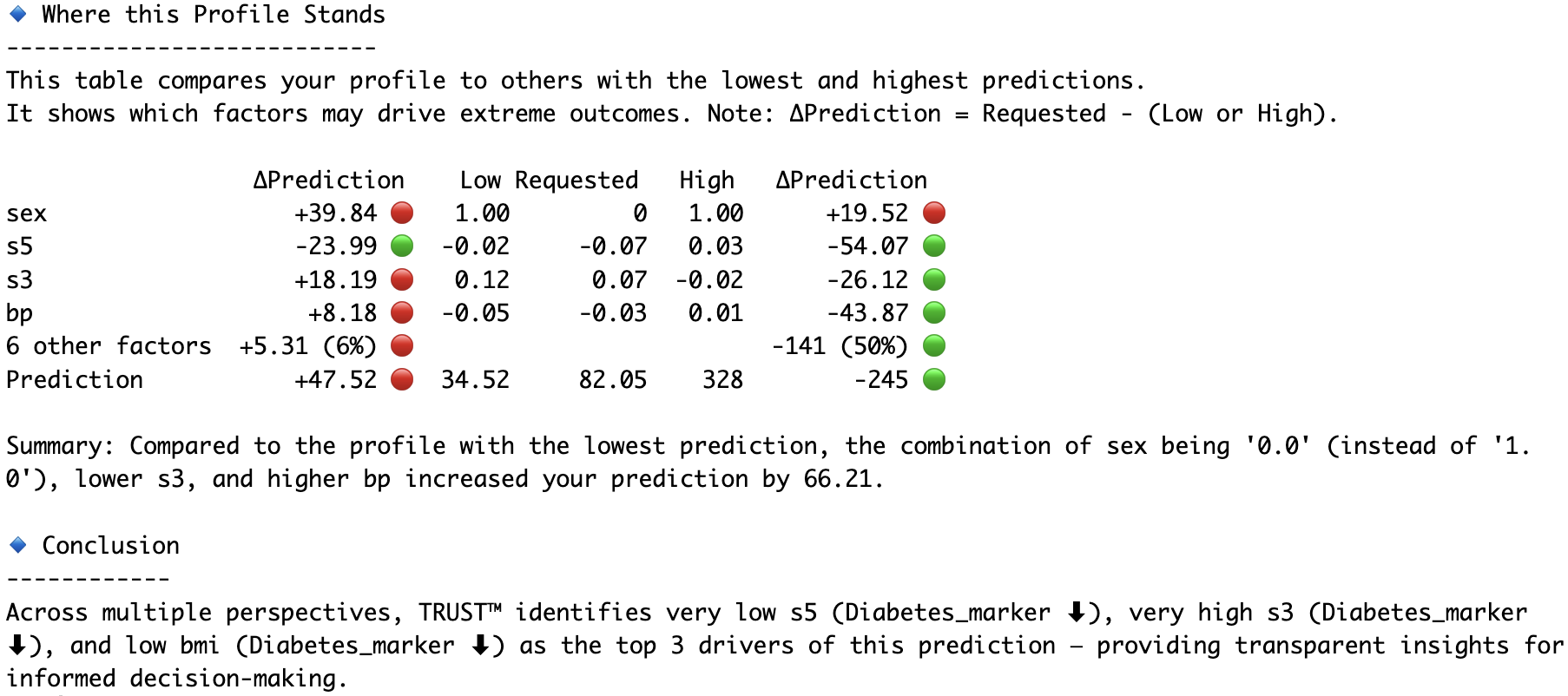
model.explain(X_test[0,:], mode="detailed", actual=y_test[0], filename="Synthetic") 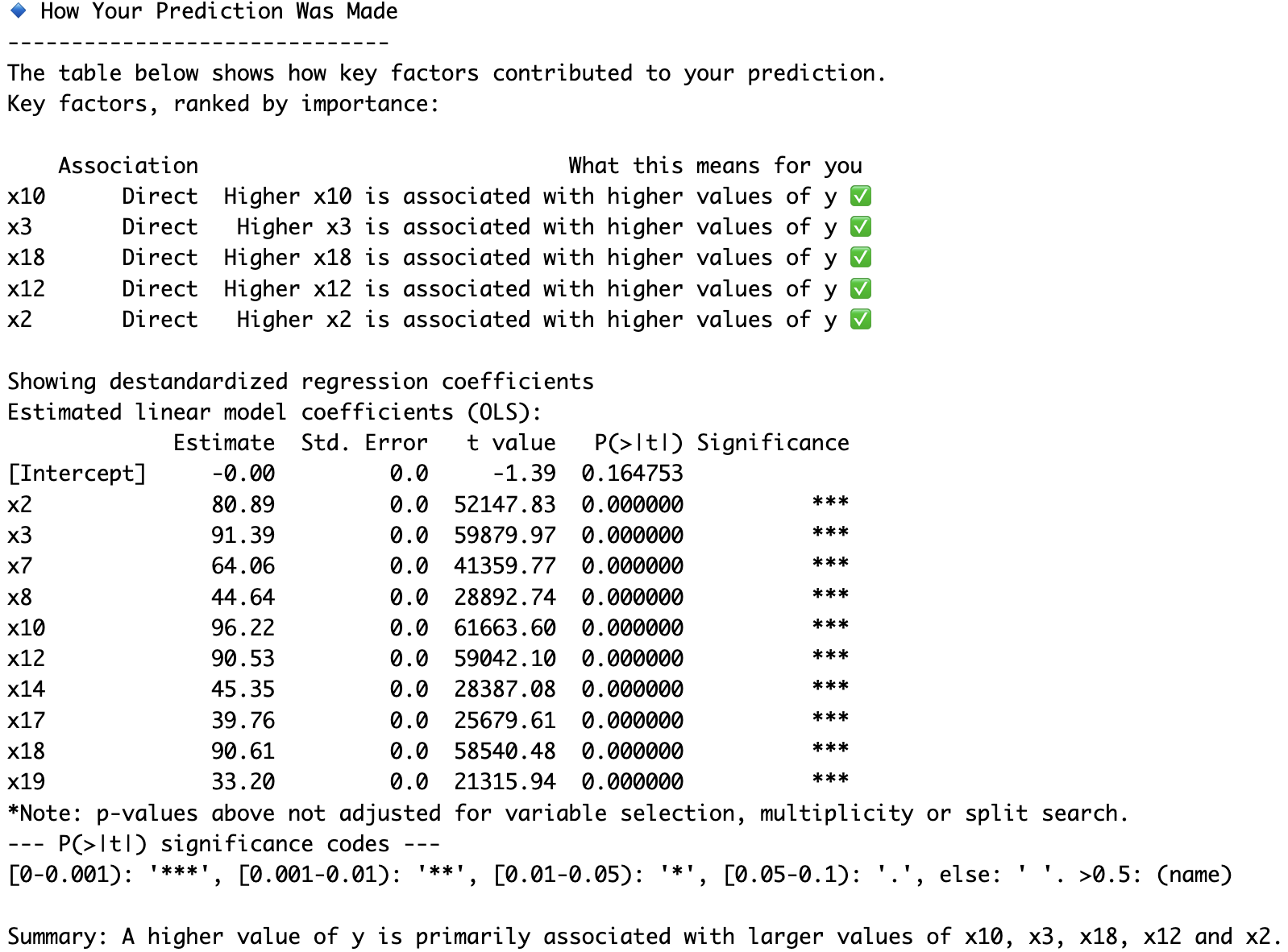
import pandas as pd
from sklearn import datasets
from sklearn.preprocessing import LabelEncoder

Diabetes = pd.DataFrame(datasets.load_diabetes().data)
Diabetes.columns = datasets.load_diabetes().feature_names
diab_target = datasets.load_diabetes().target
Diabetes.insert(len(Diabetes.columns), "Disease_marker", diab_target)
Diabetes_X = Diabetes.iloc[:,:-1]
# Binary encoding (0/1) for 'sex'
le = LabelEncoder()
Diabetes_X.loc[:, 'sex'] = le.fit_transform(Diabetes_X['sex']).astype(str)
Diabetes_y = Diabetes.iloc[:,-1]
RLT_Diabetes = TRUST(max_depth=1)
RLT_Diabetes.fit(Diabetes_X,Diabetes_y)
y_pred_TRUST = RLT_Diabetes.predict(Diabetes_X)
# Tree plotting requires Graphviz to be installed in your system path
# You can use e.g. Homebrew: brew install graphviz or Conda: conda install -c conda-forge graphviz
RLT_Diabetes.plot_tree("Diabetes") #will save "tree_plot_Diabetes.png" in your working directory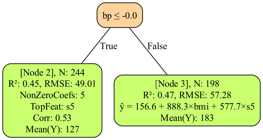
# Obtain variable importance with 2 different methods: Ghost and permutation
RLT_Diabetes.varImp(Diabetes_X, Diabetes_y, corAnalysis=True, filename="Diabetes") #Ghost method
RLT_Diabetes.varImpPerm(Diabetes_X, Diabetes_y, filename="Diabetes") #Permutation method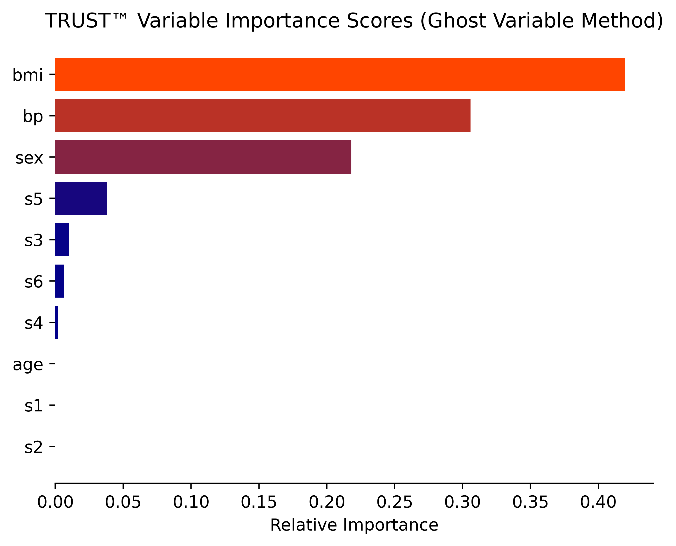
# Obtain prediction explanation for second observation
RLT_Diabetes.explain(Diabetes_X.iloc[1,:], aim="decrease", actual=Diabetes_y[1], filename="Diabetes")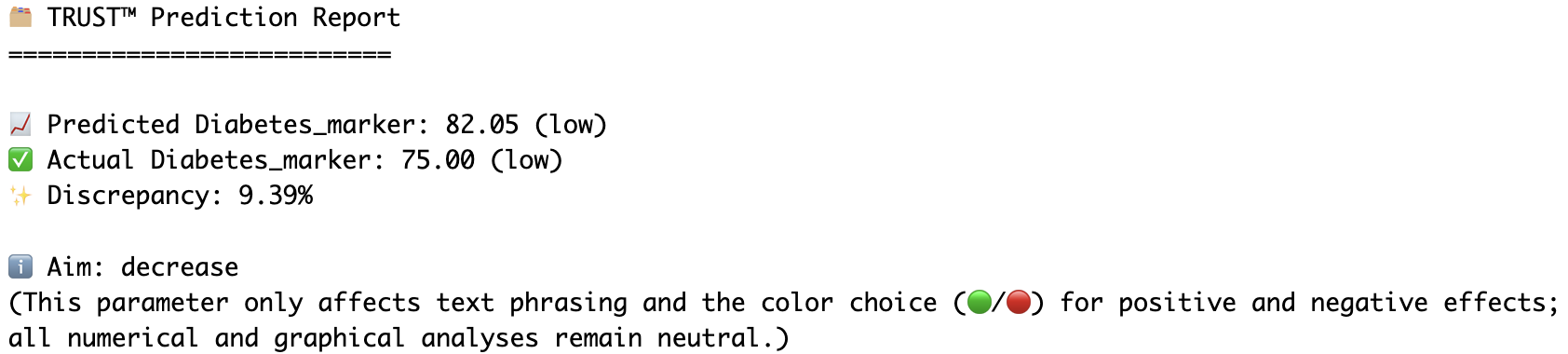
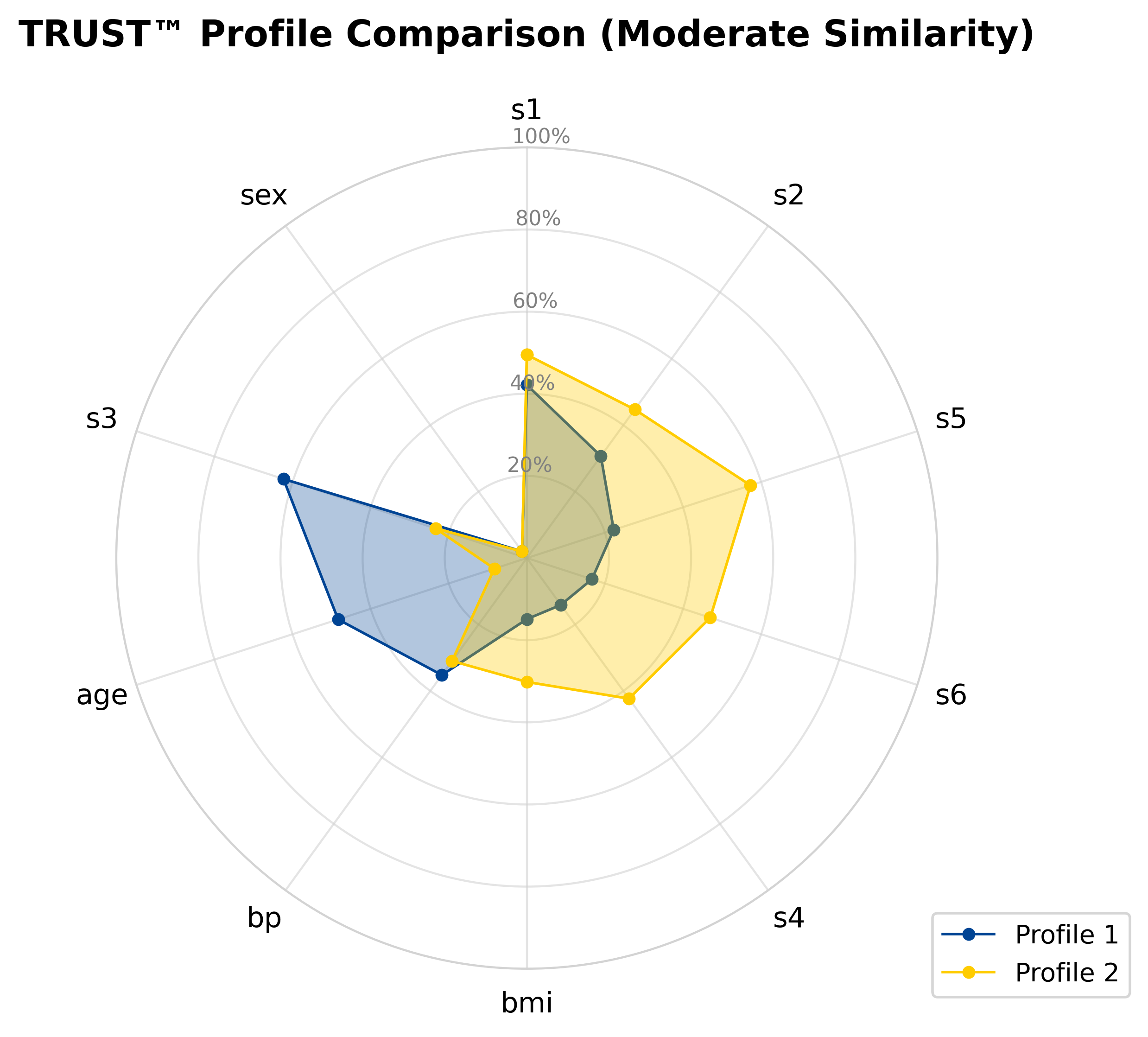
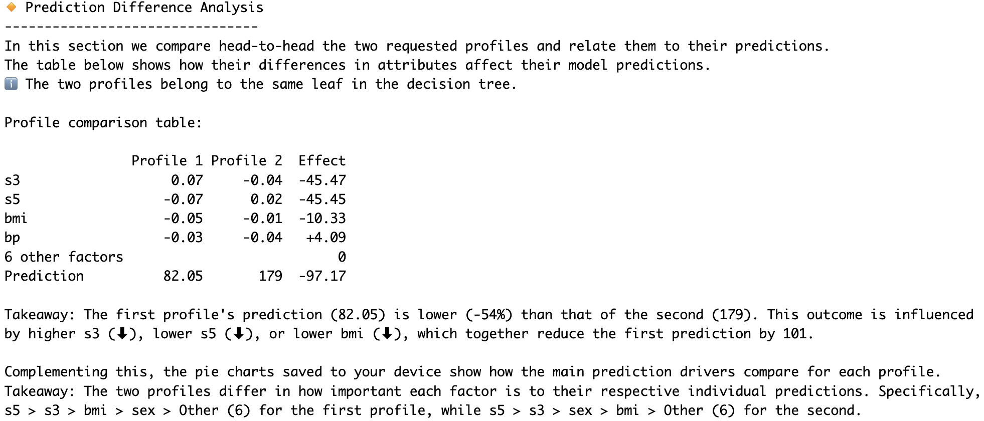
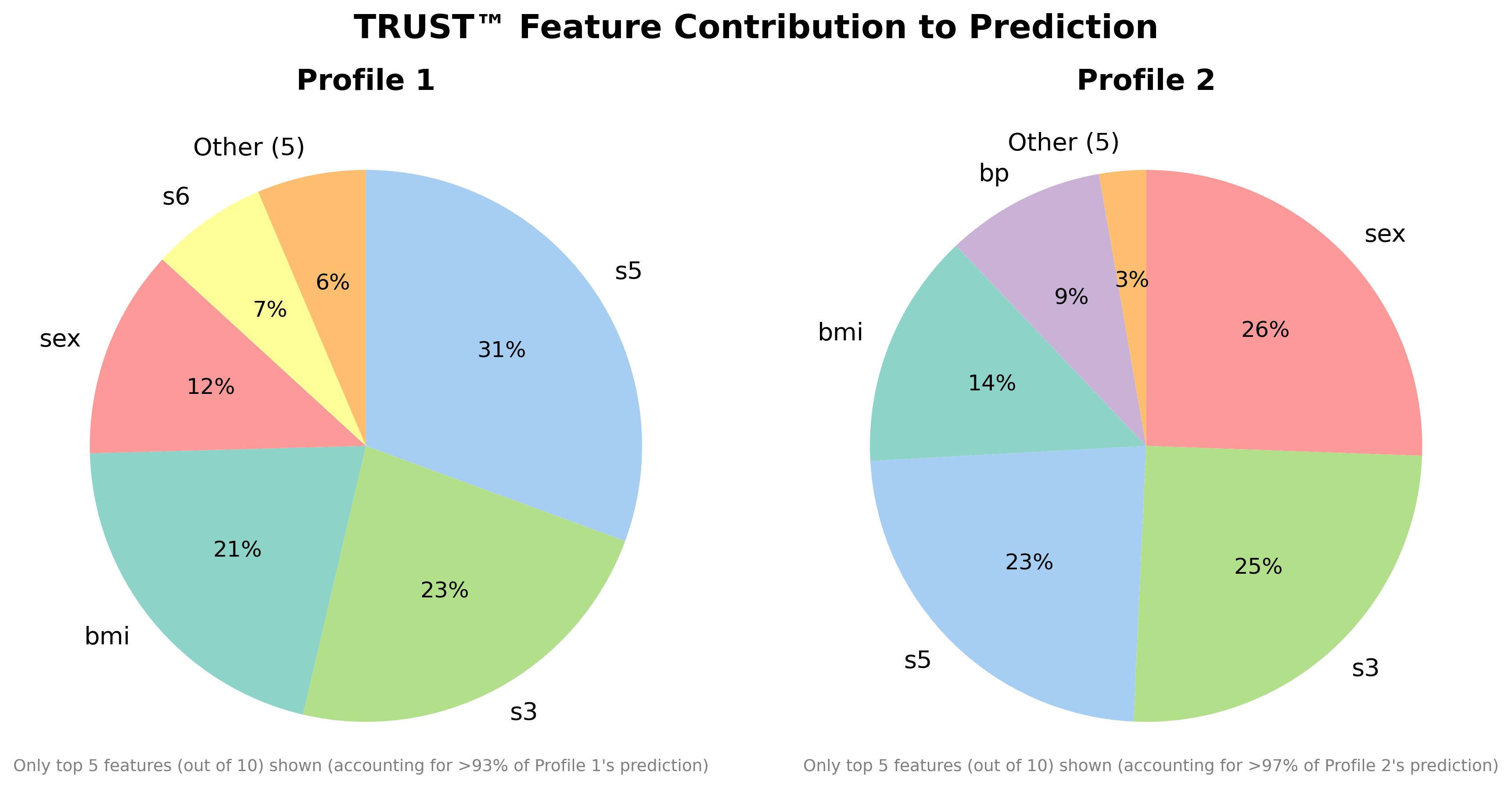
# Compare the second and fourth observations head-to-head
RLT_Diabetes.compare(Diabetes_X.iloc[1,:], Diabetes_X.iloc[3,:], filename="Diabetes")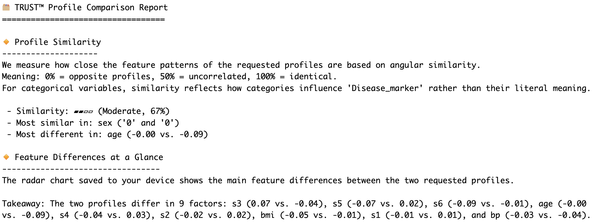
- Medical Insurance Charges (1.82M views, 360K downloads)
- Life Satisfaction in the EU (own contribution)
This software is provided under a Proprietary - Permissive Binary Only license. See LICENSE.txt for details.
For more details, documentation, and information about the full upcoming 'pro' version of the TRUST™ algorithm, please visit our official website:
https://adc-trust-ai.github.io/trust/
Further details about the TRUST™ algorithm can be found in our preprint on arXiv:
https://www.arxiv.org/abs/2506.15791
Copyright © 2025 Albert Dorador Chalar. All rights reserved. TRUST™ is a trademark of Albert Dorador Chalar.