fastcpd

Fast change point detection in Python

A Python library for detecting change points in time series and sequential data using PELT (Pruned Exact Linear Time) and SeGD (Sequential Gradient Descent) algorithms.

Documentation: https://zhangxiany-tamu.github.io/fastcpd_Python/

Now available on Test PyPI for testing! Try it with:

pip install --index-url https://test.pypi.org/simple/ --extra-index-url https://pypi.org/simple/ pyfastcpd

Features:

• Parametric models: mean/variance, GLM (binomial/Poisson), linear/LASSO regression, ARMA/GARCH
• Nonparametric methods: rank-based and RBF kernel
• C++ implementation for core models, Python for specialized models
• Comprehensive evaluation metrics and dataset generators
• Optional Numba acceleration for GLM models

Installation

From Test PyPI (Recommended for Testing)

The package is available on Test PyPI as pyfastcpd:

# Install Armadillo first (required for building C++ extension)
# macOS:
brew install armadillo

# Ubuntu/Debian:
# sudo apt-get install libarmadillo-dev

# Then install pyfastcpd
pip install --index-url https://test.pypi.org/simple/ --extra-index-url https://pypi.org/simple/ pyfastcpd

Note: Test PyPI currently only has source distribution (no pre-built wheels). You must install Armadillo before running pip install.

From Source (For Development)

System Requirements for Building from Source:

• Python ≥ 3.8
• C++17 compiler
• Armadillo library (required for C++ compilation):
  • macOS: brew install armadillo
  • Ubuntu/Debian: sudo apt-get install libarmadillo-dev

# Install Armadillo first (required!)
# macOS:
brew install armadillo

# Ubuntu/Debian:
# sudo apt-get install libarmadillo-dev

# Clone repository
git clone https://github.com/zhangxiany-tamu/fastcpd_Python.git
cd fastcpd_Python

# Install with editable mode
pip install -e .

# Optional extras for examples/benchmarks/time series notebooks
pip install -e .[dev,test,benchmark,timeseries]

# Optional: Install Numba for 7-14x GLM speedup
pip install numba

Supported Platforms: Linux, macOS (Windows support is experimental)

Quick Start

Mean Change Detection

import numpy as np
import matplotlib.pyplot as plt
from fastcpd.segmentation import mean

# Generate data with mean changes
np.random.seed(42)
data = np.concatenate([
    np.random.normal(0, 1, 100),
    np.random.normal(5, 1, 100),
    np.random.normal(2, 1, 100)
])

# Detect change points
result = mean(data, beta="MBIC")
print(f"Detected change points: {result.cp_set}")
# Output: [100, 200]

# Plot
plt.figure(figsize=(12, 4))
plt.plot(data, label='Data', linewidth=1)
for cp in result.cp_set:
    plt.axvline(cp, color='red', linestyle='--', linewidth=2, label='Detected Change Point')
plt.xlabel('Time')
plt.ylabel('Value')
plt.title('Mean Change Detection Example')
plt.legend()
plt.grid(True, alpha=0.3)
plt.tight_layout()
plt.savefig('mean_change_detection.png', dpi=150)
plt.show()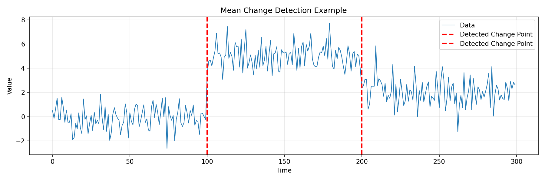

Variance Change Detection

import numpy as np
import matplotlib.pyplot as plt
from fastcpd.segmentation import variance

# Generate data with variance changes
np.random.seed(42)
data = np.concatenate([
    np.random.normal(0, 0.5, 100),
    np.random.normal(0, 2.5, 100),
    np.random.normal(0, 0.5, 100)
])

# Detect change points
result = variance(data, beta="MBIC")
print(f"Detected change points: {result.cp_set}")
# Output: [100, 200]

# Plot
plt.figure(figsize=(12, 4))
plt.plot(data, label='Data', linewidth=1, color='green')
for cp in result.cp_set:
    plt.axvline(cp, color='red', linestyle='--', linewidth=2, label='Detected Change Point')
plt.xlabel('Time')
plt.ylabel('Value')
plt.title('Variance Change Detection Example')
plt.legend()
plt.grid(True, alpha=0.3)
plt.tight_layout()
plt.savefig('variance_change_detection.png', dpi=150)
plt.show()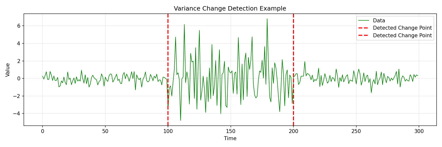

For combined mean and variance changes, use meanvariance(data, beta="MBIC")

AR Model Change Detection

Detect changes in autoregressive model parameters:

import numpy as np
import matplotlib.pyplot as plt
from fastcpd.segmentation import ar

# Generate AR(1) data with coefficient change
np.random.seed(100)
n = 300

# First segment: AR(1) with φ = 0.8
data1 = np.zeros(150)
for i in range(1, 150):
    data1[i] = 0.8 * data1[i-1] + np.random.normal(0, 0.8)

# Second segment: AR(1) with φ = -0.7
data2 = np.zeros(150)
for i in range(1, 150):
    data2[i] = -0.7 * data2[i-1] + np.random.normal(0, 0.8)

data = np.concatenate([data1, data2])

# Detect change points
result = ar(data, p=1, beta="MBIC")
print(f"Detected change points: {result.cp_set}")
# Output: [150]

# Plot
plt.figure(figsize=(12, 4))
plt.plot(data, label='AR(1) Data', linewidth=1, alpha=0.7)
plt.axvline(150, color='gray', linestyle=':', linewidth=2, label='True Change Point')
for cp in result.cp_set:
    plt.axvline(cp, color='red', linestyle='--', linewidth=2, label='Detected Change Point')
plt.xlabel('Time')
plt.ylabel('Value')
plt.title('AR Model Change Point Detection')
plt.text(75, plt.ylim()[1]*0.9, 'AR(1): φ=0.8', ha='center')
plt.text(225, plt.ylim()[1]*0.9, 'AR(1): φ=-0.7', ha='center')
plt.legend()
plt.grid(True, alpha=0.3)
plt.tight_layout()
plt.savefig('ar_change_detection.png', dpi=150)
plt.show()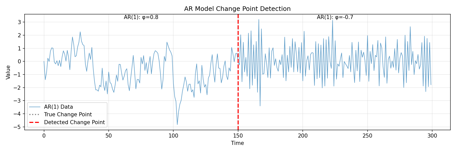

GLM and Regression Models

from fastcpd import fastcpd

# Logistic regression (binomial GLM)
# Data format: first column = response, remaining = predictors
data = np.column_stack([y, X])
result = fastcpd(data, family="binomial", beta="MBIC")

# Poisson regression
result = fastcpd(data, family="poisson", beta="MBIC")

# Linear regression
result = fastcpd(data, family="lm", beta="MBIC")

# LASSO (sparse regression)
result = fastcpd(data, family="lasso", beta="MBIC")

Time Series Models

# ARMA(p,q) - requires statsmodels
result = fastcpd(data, family='arma', order=[1, 1], beta='MBIC')

# GARCH(p,q) - requires arch package
result = fastcpd(data, family='garch', order=[1, 1], beta=2.0)

Nonparametric Methods

from fastcpd.segmentation import rank, rbf

# Rank-based (distribution-free, monotonic-invariant)
result = rank(data, beta=50.0)

# RBF kernel (detects distributional changes via kernel methods)
result = rbf(data, beta=30.0)

Algorithm Options

The vanilla_percentage parameter controls the PELT/SeGD hybrid:

# For GLM models only
result = fastcpd(data, family="binomial", vanilla_percentage=0.5)
# 0.0 = pure SeGD (fast), 1.0 = pure PELT (accurate), 'auto' = adaptive

Supported Models

Family	Description	Implementation
mean	Mean change detection	C++ (fast)
variance	Variance/covariance change	C++ (fast)
meanvariance	Combined mean & variance	C++ (fast)
binomial	Logistic regression	Python + Numba
poisson	Poisson regression	Python + Numba
lm	Linear regression	Python
lasso	L1-penalized regression	Python
ar	AR(p) autoregressive	Python
var	VAR(p) vector autoregressive	Python
arma	ARMA(p,q) time series	Python (statsmodels)
garch	GARCH(p,q) volatility	Python (arch)
rank	Rank-based (nonparametric)	Python
rbf	RBF kernel (nonparametric)	Python (RFF)

Evaluation Metrics & Datasets

Built-in Metrics:

• Precision, Recall, F1-Score
• Hausdorff distance, Covering metric
• Annotation error, One-to-one correspondence

Dataset Generators:

• Mean/variance shifts
• GLM coefficient changes
• Trend changes with multiple types
• Periodic/seasonal patterns
• Rich metadata for reproducibility

See examples/ and notebooks/ for demonstrations.

Building from Source

# Install system dependencies (macOS)
brew install armadillo

# Install system dependencies (Ubuntu/Debian)
sudo apt-get install libarmadillo-dev

# Clone and install
git clone https://github.com/zhangxiany-tamu/fastcpd_Python.git
cd fastcpd_Python
pip install -e .

# Optional: Install Numba for 7-14x GLM speedup
pip install numba

Related Projects

• fastcpd R package - Original R implementation
• fastcpd Web App - Interactive Shiny interface

License

This project is licensed under the MIT License - see the LICENSE file for details.

Documentation & Support

• Documentation: https://zhangxiany-tamu.github.io/fastcpd_Python/
• Issues: GitHub Issues
• Email: zhangxiany@stat.tamu.edu