Topic: Quadratures

About Quadratures

Suppose we have a digitized voltage signal where the $n^\text{th}$ value is $V_n$. Several device interfaces are equipped with an interface for estimating the "X and Y quadratures" of this data at frequency $f$. Mathematically, these quadratures are defined as

$X=\frac{\sum_{n}V_{n}\cos(2\pi ft_{n})}{\sum_{n}\cos^{2}(2\pi ft_{n})}$

and

$Y=\frac{\sum_{n}V_{n}\sin(2\pi ft_{n})}{\sum_{n}\sin^{2}(2\pi ft_{n})}$

where $t_n$ is the time of the $n^\text{th}$ data point. The factor in the denominator ensures that, if our time-domain signal is oscillatory with form

$V_n=V_0\cos(2\pi ft_n + \phi_0)=V_0\cos(\phi_0)\cos(ft_n)-V_0\sin(\phi_0)\sin(ft_n)$

(and the data set contains an integer number of periods at $f$), this will produce quadratures

$X=V_0\cos\phi_0$

and

$Y=-V_0\sin\phi_0$

allowing you to estimate the magnitude and phase of a single frequency component.

The Graphical Interface

The interface for estimating quadratures looks similar to this:

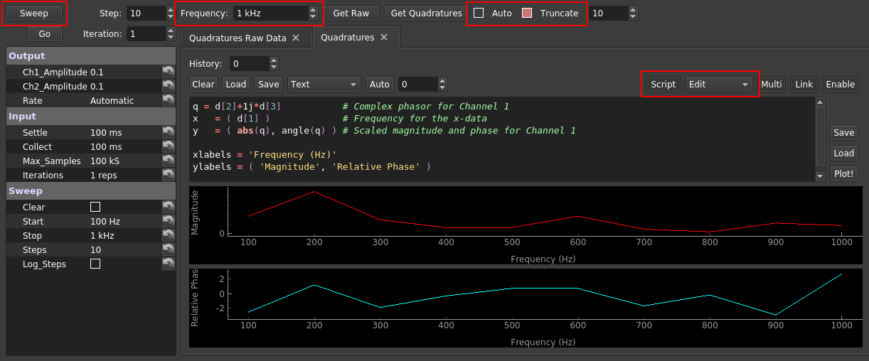
As you can see, there are a lot going on, and I've highlighted the three most important. First, if "Auto" is checked, whenever a new data set is collected, it will be transferred to the "Quadratures Raw Data" tab, its quadratures will be estimated for the shown frequency, and the resulting quadratures will be appended to the shown Databox Plotter. You probably want to adjust the plot script (red box on right) to visualize quantities of interest; the shown example plots the magnitude and phase of the first channel. Another common example is to adjust the phase of the first channels quadrature to be relative to the second channel, which can be accomplished with this:

q1  = d[2]+1j*d[3]             # Complex phasor for Channel 1
q2  = d[4]+1j*d[5]             # Complex phasor for Channel 2
q1r = q1*abs(q2)/q2            # q1 but with phase relative to that of q2
x   = ( d[1] )                 # Frequency for the x-data
y   = ( abs(q1r), angle(q1r) ) # Scaled magnitude and phase for Channel 1

xlabels = 'Frequency (Hz)'
ylabels = ( 'Magnitude', 'Relative Phase' )

We emphasize that it is important to ensure the incoming data sets contains an integer number of periods at ![f], or this interpretation is no longer valid. To assist, if "Truncate" is checked, it will automatically reduce the size of the incoming data set such that it contains an integer number of periods.

Finally, the "Sweep" button allows you to measure quadratures at different frequencies. Specifically it:

1. Sets all outputs to cosines of the specified amplitudes, and sets the frequency to that shown in "Sweep/Start".

2. Sends the waveform to the physical outputs and waits a time "Input/Settle" for the system to settle.

3. Collects an integer number of periods exceeding "Input/Collect" (provided the number of samples does not exceed "Input/Max_Samples"), and calculates the quadratures. This step is repeated as shown in "Input/Iterations".

4. Sets the output frequencies to the next value and returns to step 2.

On some interfaces, steps 2-3 can be performed with a "Go" button. As usual, you can find out more about each control by hovering your mouse.

Scripting

quadratures follows the same naming conventions as the rest of our software, with a minimally cluttered name space that can be navigated with code completion. Here are some examples:

• quadratures.plot_raw is the raw Databox Plotter.
• quadratures.plot_quadratures is the quadratures Databox Plotter.
• quadratures.checkbox_auto and quadratures.checkbox_truncate are the check boxes mentioned above.
• quadratures.button_sweep is the "Sweep" button.
• quadratures.settings is the Tree Dictionary on the left.
• etc...